Implementing gradient descent

Okay, now we know how to update our weights:

\Delta w_{ij} = \eta * \delta_j * x_i ,

You've seen how to implement that for a single update, but how do we translate that code to calculate many weight updates so our network will learn?

As an example, I'm going to have you use gradient descent to train a network on graduate school admissions data (found at http://www.ats.ucla.edu/stat/data/binary.csv). This dataset has three input features: GRE score, GPA, and the rank of the undergraduate school (numbered 1 through 4). Institutions with rank 1 have the highest prestige, those with rank 4 have the lowest.

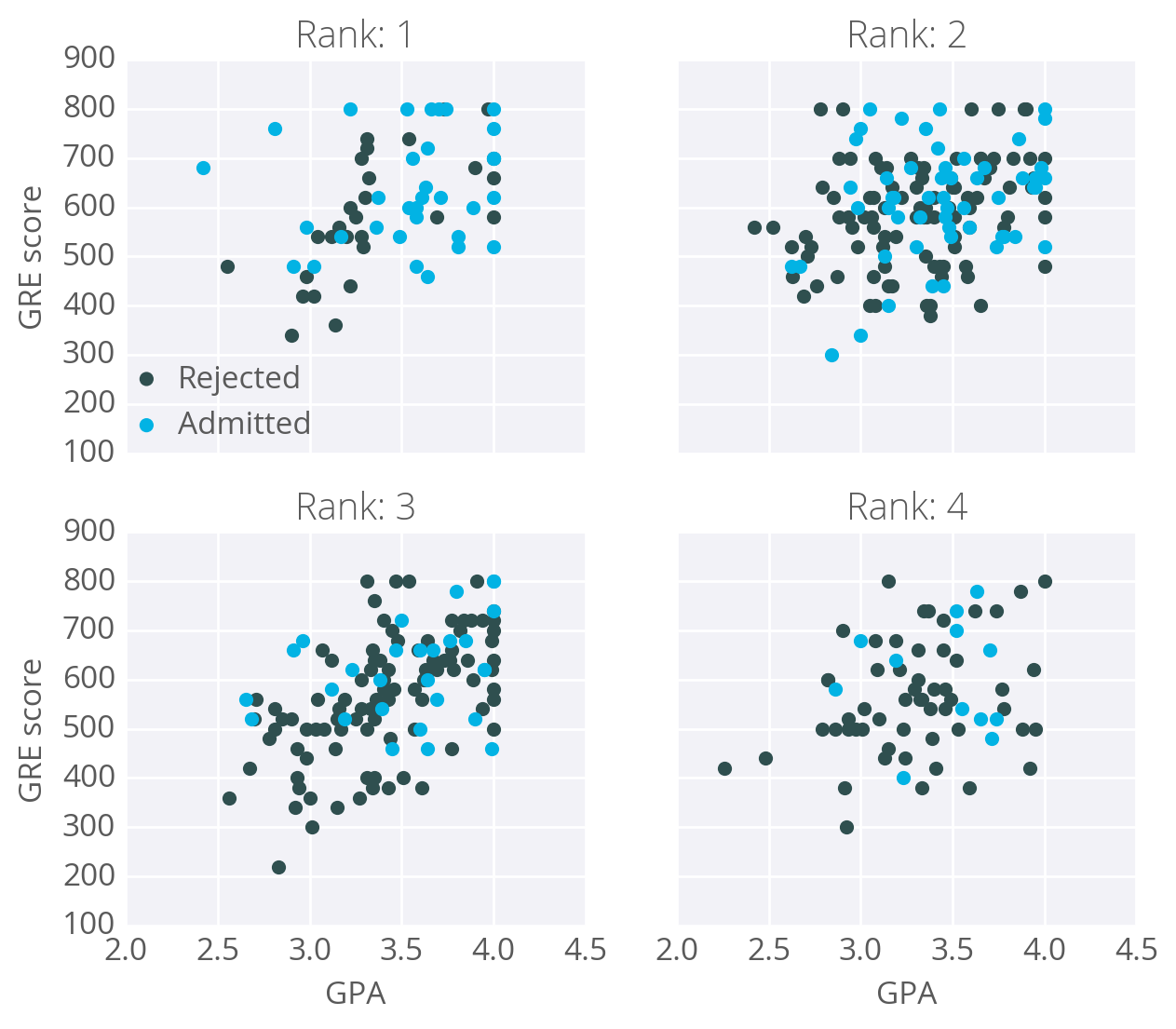
The goal here is to predict if a student will be admitted to a graduate program based on these features. For this, we'll use a network with one output layer with one unit. We'll use a sigmoid function for the output unit activation.

Data cleanup

You might think there will be three input units, but we actually need to transform the data first. The rank feature is categorical, the numbers don't encode any sort of relative values. Rank 2 is not twice as much as rank 1, rank 3 is not 1.5 more than rank 2. Instead, we need to use dummy variables to encode rank, splitting the data into four new columns encoded with ones or zeros. Rows with rank 1 have one in the rank 1 dummy column, and zeros in all other columns. Rows with rank 2 have one in the rank 2 dummy column, and zeros in all other columns. And so on.

We'll also need to standardize the GRE and GPA data, which means to scale the values such that they have zero mean and a standard deviation of 1. This is necessary because the sigmoid function squashes really small and really large inputs. The gradient of really small and large inputs is zero, which means that the gradient descent step will go to zero too. Since the GRE and GPA values are fairly large, we have to be really careful about how we initialize the weights or the gradient descent steps will die off and the network won't train. Instead, if we standardize the data, we can initialize the weights easily and everyone is happy.

This is just a brief run-through, you'll learn more about preparing data later. If you're interested in how I did this, check out the data_prep.py file in the programming exercise below.

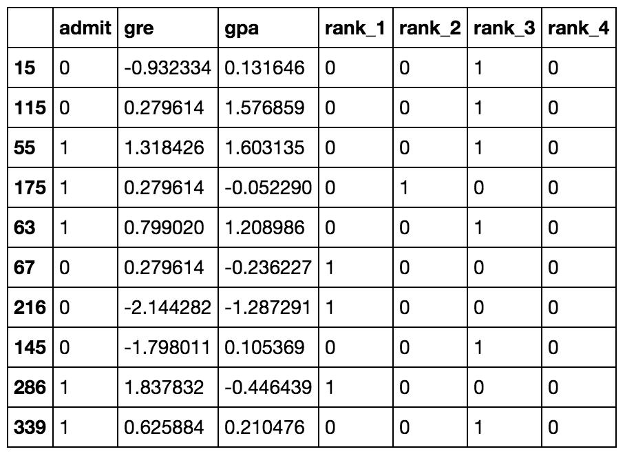
Ten rows of the data after transformations.

Now that the data is ready, we see that there are six input features: gre, gpa, and the four rank dummy variables.

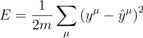
Mean Square Error

We're going to make a small change to how we calculate the error here. Instead of the SSE, we're going to use the mean of the square errors (MSE). Now that we're using a lot of data, summing up all the weight steps can lead to really large updates that make the gradient descent diverge. To compensate for this, you'd need to use a quite small learning rate. Instead, we can just divide by the number of records in our data, m to take the average. This way, no matter how much data we use, our learning rates will typically be in the range of 0.01 to 0.001. Then, we can use the MSE (shown below) to calculate the gradient and the result is the same as before, just averaged instead of summed.

Here's the general algorithm for updating the weights with gradient descent:

Set the weight step to zero: \Delta w_i = 0
For each record in the training data:
- Make a forward pass through the network, calculating the output \hat y = f(\sum_i w_i x_i)
- Calculate the error term for the output unit, \delta = (y - \hat y) * f'(\sum_i w_i x_i)
- Update the weight step \Delta w_i = \Delta w_i + \delta x_i
Update the weights w_i = w_i + \eta \Delta w_i / m where \eta is the learning rate and m is the number of records. Here we're averaging the weight steps to help reduce any large variations in the training data.
Repeat for e epochs.

You can also update the weights on each record instead of averaging the weight steps after going through all the records.

Remember that we're using the sigmoid for the activation function,
f(h) = 1/(1+e^{-h})

And the gradient of the sigmoid is
f'(h) = f(h) (1 - f(h))

where h is the input to the output unit,

h = \sum_i w_i x_i

Implementing with NumPy

For the most part, this is pretty straightforward with NumPy.

First, you'll need to initialize the weights. We want these to be small such that the input to the sigmoid is in the linear region near 0 and not squashed at the high and low ends. It's also important to initialize them randomly so that they all have different starting values and diverge, breaking symmetry. So, we'll initialize the weights from a normal distribution centered at 0. A good value for the scale is 1/\sqrt{n} where n is the number of input units. This keeps the input to the sigmoid low for increasing numbers of input units.

weights = np.random.normal(scale=1/n_features**.5, size=n_features)

NumPy provides a function np.dot() that calculates the dot product of two arrays, which conveniently calculates h for us. The dot product multiplies two arrays element-wise, the first element in array 1 is multiplied by the first element in array 2, and so on. Then, each product is summed.

# input to the output layer
output_in = np.dot(weights, inputs)

And finally, we can update \Delta w_i and w_i by incrementing them with weights += ... which is shorthand for weights = weights + ....

Efficiency tip!

You can save some calculations since we're using a sigmoid here. For the sigmoid function, f'(h) = f(h) (1 - f(h)). That means that once you calculate f(h), the activation of the output unit, you can use it to calculate the gradient for the error gradient.

Programming exercise

Below, you'll implement gradient descent and train the network on the admissions data. Your goal here is to train the network until you reach a minimum in the mean square error (MSE) on the training set. You need to implement:

The network output: output.
The output error: error.
The error term: error_term.
Update the weight step: del_w +=.
Update the weights: weights +=.

After you've written these parts, run the training by pressing "Test Run". The MSE will print out, as well as the accuracy on a test set, the fraction of correctly predicted admissions.

Feel free to play with the hyperparameters and see how it changes the MSE.

Start Quiz:

gradient.py data_prep.py binary.csv solution.py

import numpy as np
from data_prep import features, targets, features_test, targets_test


def sigmoid(x):
    """
    Calculate sigmoid
    """
    return 1 / (1 + np.exp(-x))

# TODO: We haven't provided the sigmoid_prime function like we did in
#       the previous lesson to encourage you to come up with a more
#       efficient solution. If you need a hint, check out the comments
#       in solution.py from the previous lecture.

# Use to same seed to make debugging easier
np.random.seed(42)

n_records, n_features = features.shape
last_loss = None

# Initialize weights
weights = np.random.normal(scale=1 / n_features**.5, size=n_features)

# Neural Network hyperparameters
epochs = 1000
learnrate = 0.5

for e in range(epochs):
    del_w = np.zeros(weights.shape)
    for x, y in zip(features.values, targets):
        # Loop through all records, x is the input, y is the target

        # Note: We haven't included the h variable from the previous
        #       lesson. You can add it if you want, or you can calculate
        #       the h together with the output

        # TODO: Calculate the output
        output = None

        # TODO: Calculate the error
        error = None

        # TODO: Calculate the error term
        error_term = None

        # TODO: Calculate the change in weights for this sample
        #       and add it to the total weight change
        del_w += 0

    # TODO: Update weights using the learning rate and the average change in weights
    weights += 0

    # Printing out the mean square error on the training set
    if e % (epochs / 10) == 0:
        out = sigmoid(np.dot(features, weights))
        loss = np.mean((out - targets) ** 2)
        if last_loss and last_loss < loss:
            print("Train loss: ", loss, "  WARNING - Loss Increasing")
        else:
            print("Train loss: ", loss)
        last_loss = loss


# Calculate accuracy on test data
tes_out = sigmoid(np.dot(features_test, weights))
predictions = tes_out > 0.5
accuracy = np.mean(predictions == targets_test)
print("Prediction accuracy: {:.3f}".format(accuracy))

import numpy as np
import pandas as pd

admissions = pd.read_csv('binary.csv')

# Make dummy variables for rank
data = pd.concat([admissions, pd.get_dummies(admissions['rank'], prefix='rank')], axis=1)
data = data.drop('rank', axis=1)

# Standarize features
for field in ['gre', 'gpa']:
    mean, std = data[field].mean(), data[field].std()
    data.loc[:,field] = (data[field]-mean)/std
    
# Split off random 10% of the data for testing
np.random.seed(42)
sample = np.random.choice(data.index, size=int(len(data)*0.9), replace=False)
data, test_data = data.ix[sample], data.drop(sample)

# Split into features and targets
features, targets = data.drop('admit', axis=1), data['admit']
features_test, targets_test = test_data.drop('admit', axis=1), test_data['admit']

admit,gre,gpa,rank
0,380,3.61,3
1,660,3.67,3
1,800,4,1
1,640,3.19,4
0,520,2.93,4
1,760,3,2
1,560,2.98,1
0,400,3.08,2
1,540,3.39,3
0,700,3.92,2
0,800,4,4
0,440,3.22,1
1,760,4,1
0,700,3.08,2
1,700,4,1
0,480,3.44,3
0,780,3.87,4
0,360,2.56,3
0,800,3.75,2
1,540,3.81,1
0,500,3.17,3
1,660,3.63,2
0,600,2.82,4
0,680,3.19,4
1,760,3.35,2
1,800,3.66,1
1,620,3.61,1
1,520,3.74,4
1,780,3.22,2
0,520,3.29,1
0,540,3.78,4
0,760,3.35,3
0,600,3.4,3
1,800,4,3
0,360,3.14,1
0,400,3.05,2
0,580,3.25,1
0,520,2.9,3
1,500,3.13,2
1,520,2.68,3
0,560,2.42,2
1,580,3.32,2
1,600,3.15,2
0,500,3.31,3
0,700,2.94,2
1,460,3.45,3
1,580,3.46,2
0,500,2.97,4
0,440,2.48,4
0,400,3.35,3
0,640,3.86,3
0,440,3.13,4
0,740,3.37,4
1,680,3.27,2
0,660,3.34,3
1,740,4,3
0,560,3.19,3
0,380,2.94,3
0,400,3.65,2
0,600,2.82,4
1,620,3.18,2
0,560,3.32,4
0,640,3.67,3
1,680,3.85,3
0,580,4,3
0,600,3.59,2
0,740,3.62,4
0,620,3.3,1
0,580,3.69,1
0,800,3.73,1
0,640,4,3
0,300,2.92,4
0,480,3.39,4
0,580,4,2
0,720,3.45,4
0,720,4,3
0,560,3.36,3
1,800,4,3
0,540,3.12,1
1,620,4,1
0,700,2.9,4
0,620,3.07,2
0,500,2.71,2
0,380,2.91,4
1,500,3.6,3
0,520,2.98,2
0,600,3.32,2
0,600,3.48,2
0,700,3.28,1
1,660,4,2
0,700,3.83,2
1,720,3.64,1
0,800,3.9,2
0,580,2.93,2
1,660,3.44,2
0,660,3.33,2
0,640,3.52,4
0,480,3.57,2
0,700,2.88,2
0,400,3.31,3
0,340,3.15,3
0,580,3.57,3
0,380,3.33,4
0,540,3.94,3
1,660,3.95,2
1,740,2.97,2
1,700,3.56,1
0,480,3.13,2
0,400,2.93,3
0,480,3.45,2
0,680,3.08,4
0,420,3.41,4
0,360,3,3
0,600,3.22,1
0,720,3.84,3
0,620,3.99,3
1,440,3.45,2
0,700,3.72,2
1,800,3.7,1
0,340,2.92,3
1,520,3.74,2
1,480,2.67,2
0,520,2.85,3
0,500,2.98,3
0,720,3.88,3
0,540,3.38,4
1,600,3.54,1
0,740,3.74,4
0,540,3.19,2
0,460,3.15,4
1,620,3.17,2
0,640,2.79,2
0,580,3.4,2
0,500,3.08,3
0,560,2.95,2
0,500,3.57,3
0,560,3.33,4
0,700,4,3
0,620,3.4,2
1,600,3.58,1
0,640,3.93,2
1,700,3.52,4
0,620,3.94,4
0,580,3.4,3
0,580,3.4,4
0,380,3.43,3
0,480,3.4,2
0,560,2.71,3
1,480,2.91,1
0,740,3.31,1
1,800,3.74,1
0,400,3.38,2
1,640,3.94,2
0,580,3.46,3
0,620,3.69,3
1,580,2.86,4
0,560,2.52,2
1,480,3.58,1
0,660,3.49,2
0,700,3.82,3
0,600,3.13,2
0,640,3.5,2
1,700,3.56,2
0,520,2.73,2
0,580,3.3,2
0,700,4,1
0,440,3.24,4
0,720,3.77,3
0,500,4,3
0,600,3.62,3
0,400,3.51,3
0,540,2.81,3
0,680,3.48,3
1,800,3.43,2
0,500,3.53,4
1,620,3.37,2
0,520,2.62,2
1,620,3.23,3
0,620,3.33,3
0,300,3.01,3
0,620,3.78,3
0,500,3.88,4
0,700,4,2
1,540,3.84,2
0,500,2.79,4
0,800,3.6,2
0,560,3.61,3
0,580,2.88,2
0,560,3.07,2
0,500,3.35,2
1,640,2.94,2
0,800,3.54,3
0,640,3.76,3
0,380,3.59,4
1,600,3.47,2
0,560,3.59,2
0,660,3.07,3
1,400,3.23,4
0,600,3.63,3
0,580,3.77,4
0,800,3.31,3
1,580,3.2,2
1,700,4,1
0,420,3.92,4
1,600,3.89,1
1,780,3.8,3
0,740,3.54,1
1,640,3.63,1
0,540,3.16,3
0,580,3.5,2
0,740,3.34,4
0,580,3.02,2
0,460,2.87,2
0,640,3.38,3
1,600,3.56,2
1,660,2.91,3
0,340,2.9,1
1,460,3.64,1
0,460,2.98,1
1,560,3.59,2
0,540,3.28,3
0,680,3.99,3
1,480,3.02,1
0,800,3.47,3
0,800,2.9,2
1,720,3.5,3
0,620,3.58,2
0,540,3.02,4
0,480,3.43,2
1,720,3.42,2
0,580,3.29,4
0,600,3.28,3
0,380,3.38,2
0,420,2.67,3
1,800,3.53,1
0,620,3.05,2
1,660,3.49,2
0,480,4,2
0,500,2.86,4
0,700,3.45,3
0,440,2.76,2
1,520,3.81,1
1,680,2.96,3
0,620,3.22,2
0,540,3.04,1
0,800,3.91,3
0,680,3.34,2
0,440,3.17,2
0,680,3.64,3
0,640,3.73,3
0,660,3.31,4
0,620,3.21,4
1,520,4,2
1,540,3.55,4
1,740,3.52,4
0,640,3.35,3
1,520,3.3,2
1,620,3.95,3
0,520,3.51,2
0,640,3.81,2
0,680,3.11,2
0,440,3.15,2
1,520,3.19,3
1,620,3.95,3
1,520,3.9,3
0,380,3.34,3
0,560,3.24,4
1,600,3.64,3
1,680,3.46,2
0,500,2.81,3
1,640,3.95,2
0,540,3.33,3
1,680,3.67,2
0,660,3.32,1
0,520,3.12,2
1,600,2.98,2
0,460,3.77,3
1,580,3.58,1
1,680,3,4
1,660,3.14,2
0,660,3.94,2
0,360,3.27,3
0,660,3.45,4
0,520,3.1,4
1,440,3.39,2
0,600,3.31,4
1,800,3.22,1
1,660,3.7,4
0,800,3.15,4
0,420,2.26,4
1,620,3.45,2
0,800,2.78,2
0,680,3.7,2
0,800,3.97,1
0,480,2.55,1
0,520,3.25,3
0,560,3.16,1
0,460,3.07,2
0,540,3.5,2
0,720,3.4,3
0,640,3.3,2
1,660,3.6,3
1,400,3.15,2
1,680,3.98,2
0,220,2.83,3
0,580,3.46,4
1,540,3.17,1
0,580,3.51,2
0,540,3.13,2
0,440,2.98,3
0,560,4,3
0,660,3.67,2
0,660,3.77,3
1,520,3.65,4
0,540,3.46,4
1,300,2.84,2
1,340,3,2
1,780,3.63,4
1,480,3.71,4
0,540,3.28,1
0,460,3.14,3
0,460,3.58,2
0,500,3.01,4
0,420,2.69,2
0,520,2.7,3
0,680,3.9,1
0,680,3.31,2
1,560,3.48,2
0,580,3.34,2
0,500,2.93,4
0,740,4,3
0,660,3.59,3
0,420,2.96,1
0,560,3.43,3
1,460,3.64,3
1,620,3.71,1
0,520,3.15,3
0,620,3.09,4
0,540,3.2,1
1,660,3.47,3
0,500,3.23,4
1,560,2.65,3
0,500,3.95,4
0,580,3.06,2
0,520,3.35,3
0,500,3.03,3
0,600,3.35,2
0,580,3.8,2
0,400,3.36,2
0,620,2.85,2
1,780,4,2
0,620,3.43,3
1,580,3.12,3
0,700,3.52,2
1,540,3.78,2
1,760,2.81,1
0,700,3.27,2
0,720,3.31,1
1,560,3.69,3
0,720,3.94,3
1,520,4,1
1,540,3.49,1
0,680,3.14,2
0,460,3.44,2
1,560,3.36,1
0,480,2.78,3
0,460,2.93,3
0,620,3.63,3
0,580,4,1
0,800,3.89,2
1,540,3.77,2
1,680,3.76,3
1,680,2.42,1
1,620,3.37,1
0,560,3.78,2
0,560,3.49,4
0,620,3.63,2
1,800,4,2
0,640,3.12,3
0,540,2.7,2
0,700,3.65,2
1,540,3.49,2
0,540,3.51,2
0,660,4,1
1,480,2.62,2
0,420,3.02,1
1,740,3.86,2
0,580,3.36,2
0,640,3.17,2
0,640,3.51,2
1,800,3.05,2
1,660,3.88,2
1,600,3.38,3
1,620,3.75,2
1,460,3.99,3
0,620,4,2
0,560,3.04,3
0,460,2.63,2
0,700,3.65,2
0,600,3.89,3

import numpy as np
from data_prep import features, targets, features_test, targets_test


def sigmoid(x):
    """
    Calculate sigmoid
    """
    return 1 / (1 + np.exp(-x))

# TODO: We haven't provided the sigmoid_prime function like we did in
#       the previous lesson to encourage you to come up with a more
#       efficient solution. If you need a hint, check out the comments
#       in solution.py from the previous lecture.

# Use to same seed to make debugging easier
np.random.seed(42)

n_records, n_features = features.shape
last_loss = None

# Initialize weights
weights = np.random.normal(scale=1 / n_features**.5, size=n_features)

# Neural Network hyperparameters
epochs = 1000
learnrate = 0.5

for e in range(epochs):
    del_w = np.zeros(weights.shape)
    for x, y in zip(features.values, targets):
        # Loop through all records, x is the input, y is the target

        # Activation of the output unit
        #   Notice we multiply the inputs and the weights here 
        #   rather than storing h as a separate variable 
        output = sigmoid(np.dot(x, weights))

        # The error, the target minus the network output
        error = y - output

        # The error term
        #   Notice we calulate f'(h) here instead of defining a separate
        #   sigmoid_prime function. This just makes it faster because we
        #   can re-use the result of the sigmoid function stored in
        #   the output variable
        error_term = error * output * (1 - output)

        # The gradient descent step, the error times the gradient times the inputs
        del_w += error_term * x

    # Update the weights here. The learning rate times the 
    # change in weights, divided by the number of records to average
    weights += learnrate * del_w / n_records

    # Printing out the mean square error on the training set
    if e % (epochs / 10) == 0:
        out = sigmoid(np.dot(features, weights))
        loss = np.mean((out - targets) ** 2)
        if last_loss and last_loss < loss:
            print("Train loss: ", loss, "  WARNING - Loss Increasing")
        else:
            print("Train loss: ", loss)
        last_loss = loss


# Calculate accuracy on test data
tes_out = sigmoid(np.dot(features_test, weights))
predictions = tes_out > 0.5
accuracy = np.mean(predictions == targets_test)
print("Prediction accuracy: {:.3f}".format(accuracy))

Next Concept